Flood Simulation Using the Lattice Boltzmann Method
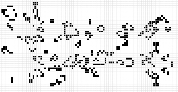
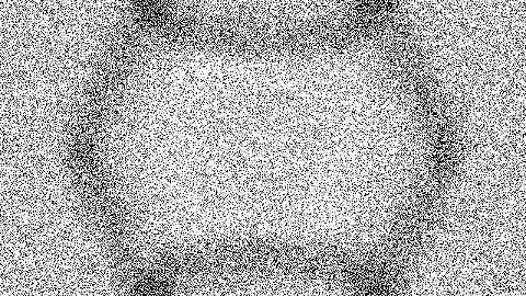
The Lattice Boltzmann Method originates from the Lattice Gas Automata which is a cellular automata designed to simulate the behavior of a gas. A cellular automata is a model characterized by a finite set of identical and synchronized automata that follow the same evolutionary rules. In a cellular automata, time is discrete and space is divided into cells, each of which is updated at each simulation step according to defined rules. In the Lattice Gas Automata these rules have been defined in order to simulate the propagation and collisions between the gas particles respecting the conservation laws. However, the simulations generated with Lattice Gas Automata contain a lot of noise due to its boolean nature. This problem leads to the birth of the Lattice Boltzmann Method, in which for each cell is stored the density in real numbers of particles moving in a certain direction.
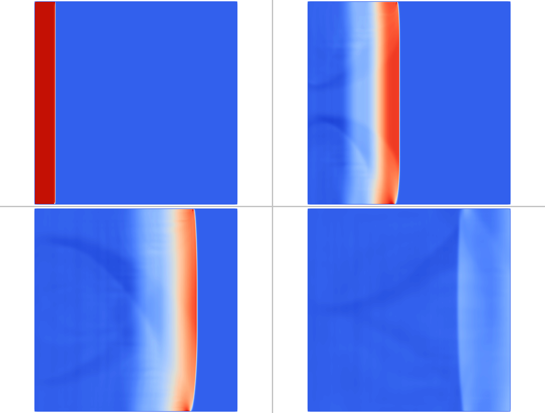
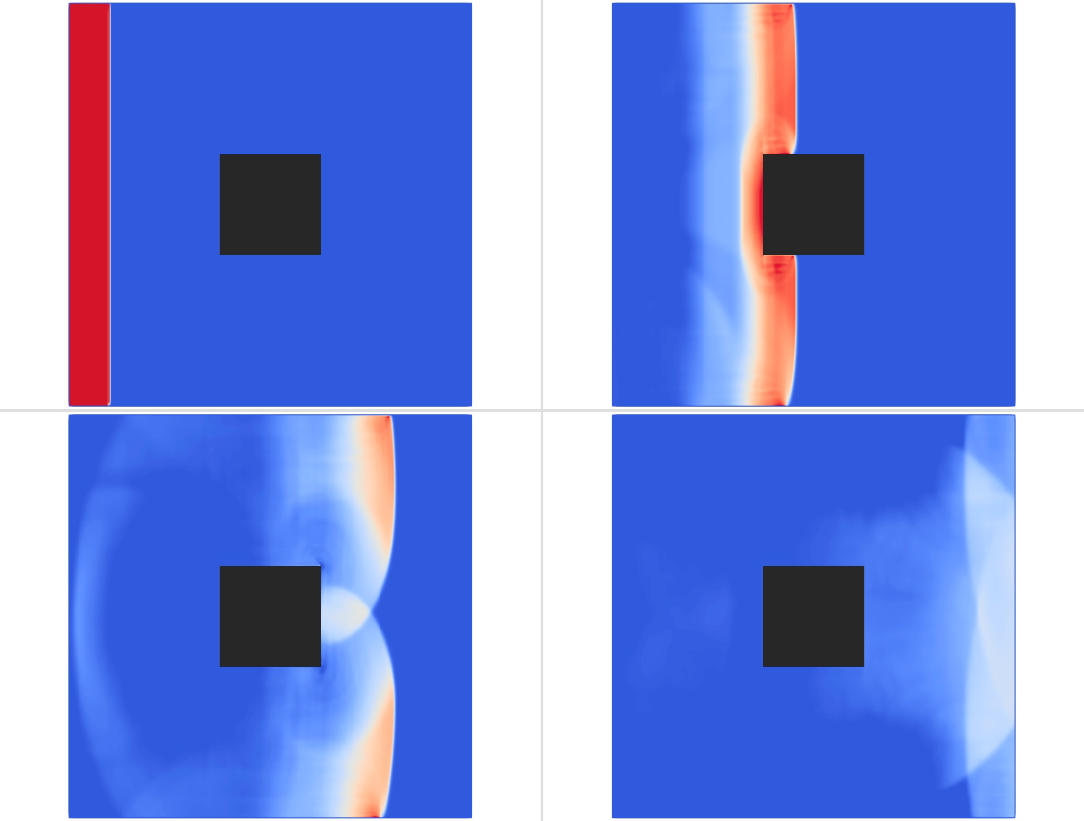
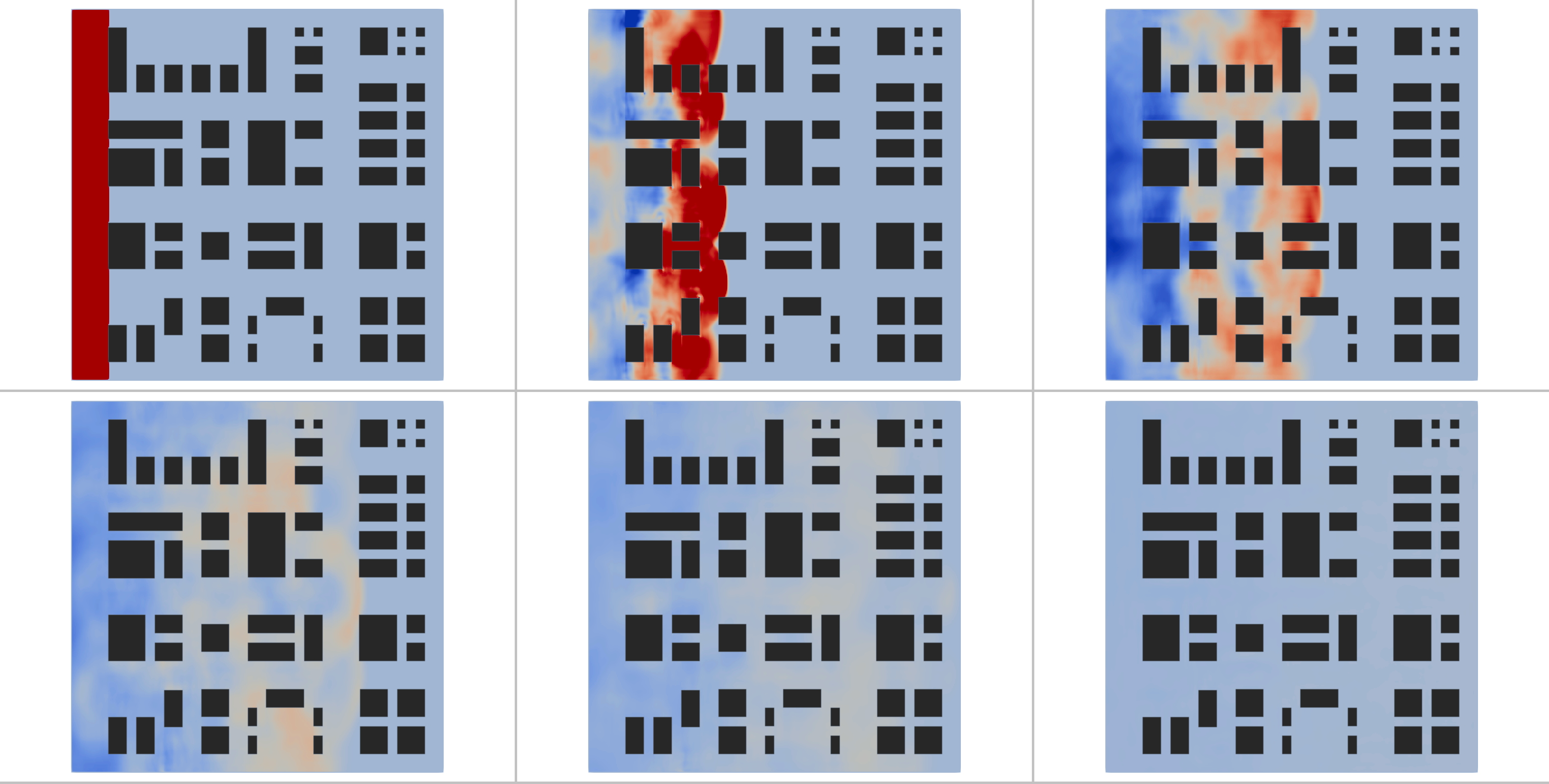
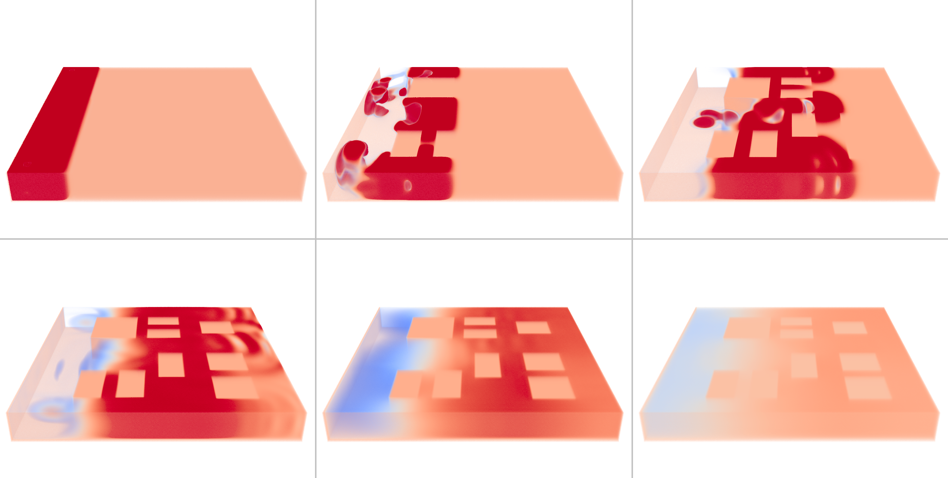
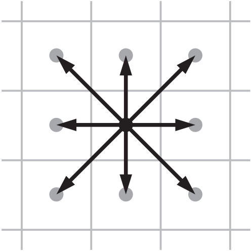
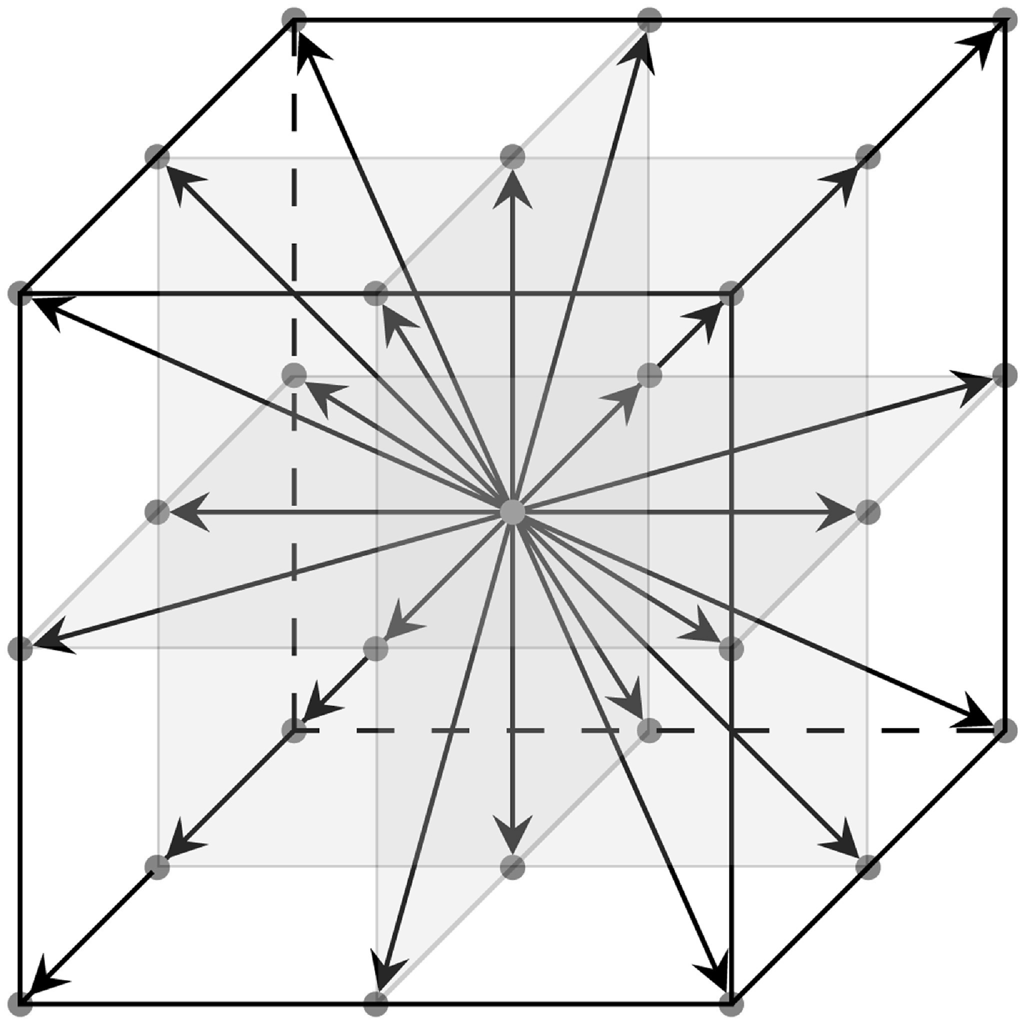
The Lattice Boltzmann Method can be applied to different lattices. A standard classification is the DnQm in which the n indicates the number of dimensions of the lattice and the m indicates the number of different discrete directions that a particle can take in motion. In this project, two simulations were carried out, one two-dimensional on a D2Q9 lattice and one three-dimensional on a D3Q27 lattice.
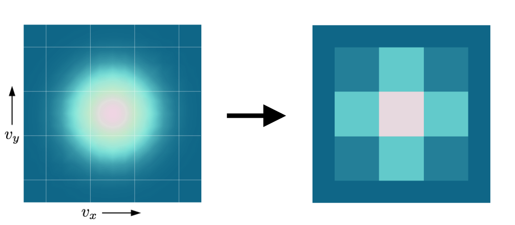
At the base of the Lattice Boltzmann Method is the Boltzmann Distribution, which represents the distribution of thermal velocities in an ideal gas.
If the fluid flows with a non-zero macroscopic velocity u, then the total velocity of each particle will be equal to the sum of u with the thermal velocity v.
Constraining this total speed to be one of the speeds allowed by the model, then we obtain the following expression.
This expression can be approximated through a Taylor series expansion obtaining the expression for the determination of the probability of the i-th velocity vector, which is the heart of the Lattice Boltzmann Method.
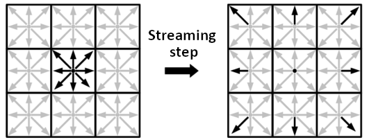
The Lattice Boltzmann's algorithm has two main steps called streaming and collision steps. In the streaming step, the particles propagate by moving in the direction of their velocity.
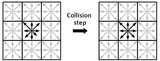
In the collision step the collisions of particles in a fluid are simulated, which make it move closer to a state of equilibrium. The density that would occur at equilibrium is then calculated and then the lattice is updated in order to bring it closer to this density by an omega factor, which depends on the viscosity of the fluid and indicates how quickly it reaches a state of equilibrium.
Results